
Author Identification using Naive Bayes Algorithm — Model Building
Written: 02 Jan 2021 by Vinayak Nayak 🏷 ["machine learning"]This post is the second in a series of three posts which aim to build a naive bayes classification algorithm in an end to end fashion. In the previous post, we looked at curating the data for this problem: We scraped dialogues for both Captain America and Iron Man from the transcripts of Captain America: The First Avenger, Iron Man and Avengers: Endgame respectively. We then processed them to remove all action/scene description cues and only retain the spoken word by both our characters and created a dataframe out of the same and saved them as csv files.
We shall now focus on building a Naive Bayes Classifier along with the working for the same from scratch. In this post, we will focus on
-
Understanding Conditional Probability
-
Understanding Bayes Theorem
-
Naive Bayes for author identification
-
Evaluating the Classification Model
Without any further ado, let’s get started!
Understanding Conditional Probability
We saw the distribution of dialogues in the previous post where around 40% of them were uttered by Captain America 60% were spoken by Iron Man. We could visualize the same in the following manner:
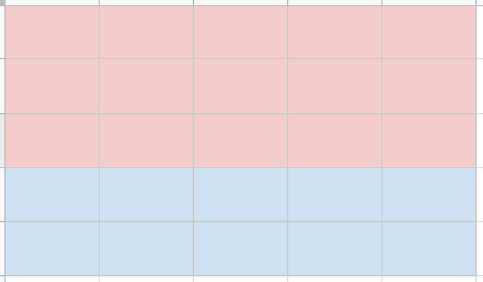
For the sake of simplicity let’s assume we have 25 dialogues, 15 of which are from Iron Man shown in red and 10 of which are spoken by Captain America which are shown in Blue; this is so as to make the graphic representative of our corpus. Now, we can say from this graphic that:
\[ P(Captain \ America) = \frac{10}{25} = \frac{2}{5} \]
\[ P(Iron \ Man) = \frac{15}{25} = \frac{3}{5} \]
Now, let’s say we look at the dialogues and we observed that the word Jarvis appears 7 times in Iron Man’s dialogues and only twice in Captain America’s dialogues. It could be shown below in this diagram
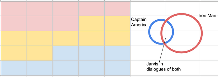
Here yellow represents the word Jarvis being present in the dialogue. We can see the same in the Venn Diagram as well.
If I had only told you that there’s a 40% chance that any given dialogue is spoken by Captain America and 60% chance that it’s uttered by Iron Man, and ask you if a given sentence is spoken by Iron Man or Captain America, you’ll most likely say Iron Man 1.5 times more often than Captain America.
But if I tell you that the sentence contains the word Jarvis, now you have an additional piece of information. You know from the distribution of sentences above that Jarvis appears more often in Iron Man’s dialogues than in Captain America’s dialogues. More specifically, we see that of all the dialogues that contain Jarvis (7), 5 of them are spoken by Iron Man and only 2 are spoken by Captain America. This means that you could very easily guess Iron Man 2.5 times more often than Captain America and you’d be right.
What just now happened is a consequence of conditional probability in action. Just by mentioning the fact that a sentence contains Jarvis, we reduced our corpus for probability computation from 25 to 7. Amongst that we then saw which character uttered that word how many times and computed the probability. In short, we conditioned on the information that the sentence has the word Jarvis in it.
\[ P(Captain \ America | Jarvis) = \frac{2}{7} \]
\[ P(Iron \ Man | Jarvis) = \frac{5}{7} \]
So, in short, we can see from the Venn Diagram that conditioning on a particular evidence reduces our sample space/ corpus space and we can better estimate the odds of an event. We can formally state that
\[ P(A | B) = \frac{P(A \cap B )}{P(B)} \]
which in our case translates to the following two expressions
\[ P(Captain \ America | Jarvis) = \frac{P(Captain \ America \cap Jarvis )}{P(Jarvis)} \]
\[ P(Iron \ Man | Jarvis) = \frac{P(Iron \ man \cap Jarvis )}{P(Jarvis)} \]
Understanding Bayes Theorem
Using the above definition of conditional probability, we can find do some algebra to come up with an equation which is colloquially known as Bayes Rule or Bayes’ Theorem.
\[ P(A | B) = \frac{P(A \cap B )}{P(B)} \]
\[ P(B | A) = \frac{P(B \cap A )}{P(A)} \]
We know that \( P(B \cup A) = P(A \cup B) \)
So, we can divide the equations and we end up getting
\[ \frac{P(A | B)}{P(B | A)} = \frac{P(A)}{P(B)} \]
or after restructuring
\[ P(A | B) = P(B | A) \times \frac{P(A)}{P(B)} \]
In the above equation, every term has a particular connotation associated with it:
P(A) — Prior probability of class A
P(B) — Prior probability of predictor B
P(B | A) — Likelihood i.e. probability of predictor given class
P(A | B) — Posterior probability of class given predictor
Bayes Rule is a very useful construct when it comes to conditional probability because in most of the cases we know the conditional probability one way but not the other (for many practical reasons) and this rule helps us figure/ realistically estimate the reverse conditional probability.
For eg. in a disease diagnostic experiment, we can estimate P(positive| disease) by doing tests on people who are only actually suffering, but finding out P(disease| positive) cannot be really calculated because testing the entire population will just be too costly & futile; especially if the disease is less prevalent.
In our case, the rule will be
\[ P(Captain \ America | Jarvis) = P(Jarvis | Captain \ America ) \times \frac{P(Captain \ America)}{P(Jarvis)} \]
The RHS conditional probability can be estimated by using the available corpus of documents and then this could be utilized during test/inference time in finding out which dialogue is more likely to have been uttered by which superhero.
But what is the Naive Bayes Algorithm and what’s so naive about it?
We have seen the Bayes Rule or Bayes Theorem above i.e.
\[ P(A | B) = P(B | A) \times \frac{P(A)}{P(B)} \]
In many cases, the B is not really singular event but a series of events happening together for eg. in our case, we can break a sentence up into individual elements/ tokens/ quantum which in the English Language would be words (in some other languages it could be phrases or even characters). The formula then looks like

If we assume that the events \(B_1, B_2, B_3, … B_n\) are independent, we can simplify the above equation and write it as follows

So, we can see that

The proportionality above can be used in order to identify the most likely class given a set of predictors. Notice how the assumption of independence turned this problem from something complex into something very modular and relatively easy.
In our case, we can take a ratio and come up with something like

If the ratio is more than 1, we can say that the narrator is more likely to be Stark than Cap and vice versa. The above representation could be shortened and represented as

where Bi are the individual tokens in sentence B Independence of tokens/words in a sentence is a naive assumption in the Naive Bayes Algorithm; hence the name. Generally in any language, there’s a co-dependence amongst different words and the order in which they appear in a sentence. For eg. in the English language, an article is always associated with a noun which means if you have an article, there’s a higher probability of the successive word being a noun than a verb or a preposition.
Despite the naive assumption, the algorithm provides a strong baseline for different tasks and is it’s time and space complexity is much less than many other algorithms out there. That’s why in most of the classification problems, data scientists first use this method to get a baseline and then improve this by using progressively complex methods like Logistic Regression, Random Forests, Multi-layer perceptron and so on…
Naive Bayes for author identification
Building on our previous work, we shall now look at how to use Naive Bayes to build a classification model for identifying the narrator of a dialogue. If you haven’t already, reading this previous post will help you get up to speed with what we are doing.
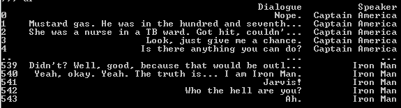
After reading in the training data, we can see it looks something like this:
Since a sentence is a certain permutation of different words, we need to first find a way to parse these. We use what is referred to as tokenization for this purpose. Let’s look at one of the ways in which we can tokenize the given sentences.
Tokenization
To use a sentence/document for any task, we first need to break it up into it’s components and then numericalize it since computers can only crunch numbers. We decide the smallest quantum which can be meaningful in case of a particular task and then break the sentence up into these quanta. In English, for our application it makes the most sense to break a sentence up at word level (in other languages you can also break it up into phrase/character level depending on the working of that respective language).
We use regular expression in order to perform the tokenization procedure. As we can see above, we have first used the compile method to define our expressions and then use these to sub (substitute for short) those expressions with the respective tokens. Eventually we lowercase all these and split on spaces to obtain our tokens.
This is a very basic way to tokenize our sentences; in order to extract the most out of a sentence, we can do much better. For eg., in English, it has become a colloquial trend to write something in all caps (uppercase) if you want to emote that you’re shouting when you type that respective word/sentence out. So, all words that are capitalized can be preceded by a special token like MAJ to capture this despite lowercasing every word in a sentence. Similarly all proper nouns are title-cased which could be captured by adding a special token like UP before a title-cased noun and so on. This is explained beautifully in these set of videos by Rachel Thomas. You can also refer this notebook and the section of special tokens in particular to understand more about this.
For now we shall resort to the simple way defined above for tokenization. We are capturing punctuation, all the words and some special combination of characters like ‘nt, ‘ll etc. which denote negation, possession etc. (even if they’re technically not words, they hold meaning in different ways and it therefore makes sense to keep them separate and utilize them like that.)
Computation of conditional probabilities
Once we have the tokens, we need to find out the prior probabilities of the two main classes (Captain America and Iron Man) and conditional probabilities of the tokens extracted from their dialogues. We can do it as follows
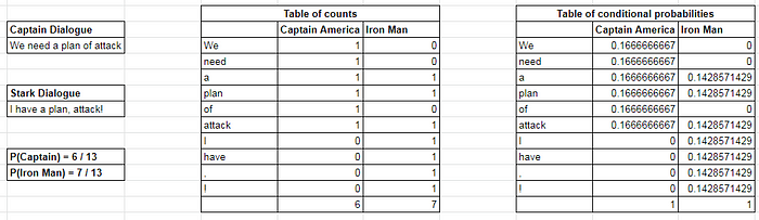
After tokenizing the sentences, we find out the counts of the individual tokens in the two classes i.e. Iron Man and Captain America and populate the table as shown above. Next we compute the conditional probability of each token by dividing the count of that token for a particular class with the total counts of tokens for that class respectively. This procedure is repeated for all the classes.
There’s two potential problems which we can run into if we use the modified formula of ratio as discussed above which are
Division by zero
In the denominator which contains terms like P(word|class), it’s possible that some probability terms evaluate to zero like in the above example we saw P(need | Iron Man) = 0.
To not encounter such problems, we could use Laplacian smoothing which modifies the conditional probability definition as follows:

We added 1 to the numerator and the term vocab_size which refers to the total number of words in our corpus. This will ensure that all the probabilities will be positive non-zero quantities.
Multiplication Underflow
When numbers with absolute value less than 1 are multiplied, their results successively go on reducing in magnitude. If we have a long sentence with many words, this could happen; in principle it’s no big deal if we were computing things with hand but computers don’t work like that.
Computers unlike mathematics are discrete and finite; multiplying a lot of small numbers will result in underflow and computer won’t be able to compute the result accurately.
We know that a log of product is the sum of logs and that is what we use for converting these product of probabilities into sum of log of probabilities. This helps circumvent this issue. If we take a log of the modified equation we discussed above we end up with

If the RHS evaluates to a positive quantity, it means the ratio on the LHS is greater than 1 which means that the dialogue is more likely to have come out of Stark’s jugular.
On the other hand, if the RHS is negative it means the ratio on the LHS is less than 1 and it is more likely that cap narrated the sentence B.
Now that we’re clear with all the terminology and theory, time to look at Naive Bayes algorithm in action.
We follow the same steps as discussed in the concepts above and we store the items in a dictionary of dictionaries as follows:
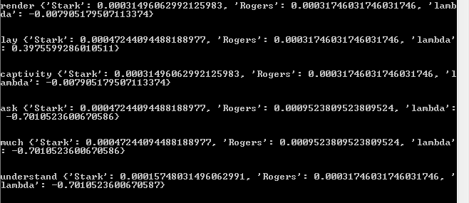
This vocabulary dictionary contains every word/vocabulary item as the key and it maps to a dictionary of conditional probabilities and log likelihood of the classes in consideration as shown above. Once we have this dictionary, we are as good as done training the model. There’s one more component of the likelihood of prior probabilities which is a part of this dictionary. It simply maps to a float value which represents log(P(A) / P(B))
In naive bayes, this dictionary mapping is all we need for making inference on any given sentence or piece of text. This function below describes how we can perform predictions using the probabilities above.
- We first tokenize the sentence to break it up into it’s individual components.
- We look up the log likelihood of each of the tokens in the sentence; if the token is absent, we use a special field xxunk and find it’s log likelihood from the probabilities dictionary.
- We sum up all these probabilities to find out the final score and add the log likelihood of prior probabilities.
- If the resulting score is positive, we classify the dialogue as belonging to Tony Stark else we say it is narrated by Steve Rogers.
Once we write this function we shall evaluate it’s performance on the same data and then evaluate it on the dialogues written from the script of Avengers Endgame to see it’s performance.
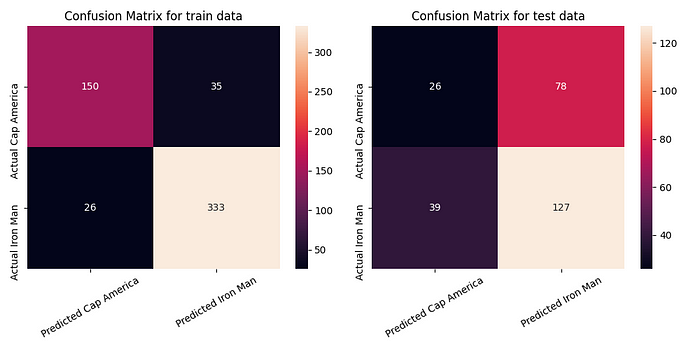
With an accuracy score of 88% on train and 57% on test data, the confusion matrix for the two sets looks as shown above. We can see that the algorithm is very sensitive to Iron Man dialogues and is good at identifying them correctly. This is to be expected because we have had an imbalanced dataset with more examples from Captain America’s dialogues and less from Iron man’s dialogues.
So, finally we now have a working implementation of naive bayes algorithm. We will store the dictionary of vocabulary shown above and use it for inference in the next post where we build an API Endpoint and dockerize the same for deployment.
I hope you enjoyed reading the post above as much as I did when writing the same. Stay tuned for the next post on deployment of this model using Flask, Flasgger and Dockers.