
Anime Recommendation System with fastai2
Written: 25 Aug 2021 by Vinayak Nayak 🏷 ["fastbook", "deep learning"]The post aims to describe what Collaborative Filtering (henceforth abbreviated as CF throughout the length of this post) is all about and subsequently elaborates on how to build a model to perform this task using fastai2. The topics covered in this post are as follows
- Introduction
- The Basic Intuition behind CF
- CF in fastai2
- The Embedding Dot Bias Model
- The Neural Network Model
- Model Interpretation & making Recommendations
- References
Introduction
In today’s world where data is oil, one way of utilising data is to perform the task of suggestion/recommendation for individuals. In this fast paced world where content is created at an astounding pace, viewers like it when they’re suggested content similar to what they’ve seen before.
In order to do so, the choices, likes, tastes etc. of the users are recorded in the form of ratings or a score which is typically bound in a finite range (most commonly 0–5 or 0–10) where 0 represents that the user strongly disliked the content and 5 or 10 represent that the user found the content very entertaining and to his liking.
Using this data in order to figure out what to next to suggest to a user is what collaborative filtering is all about. In place of user-anime or user-movie it could be anything like consumer-product or user-news article or subscriber-social media posts and so on.
The more feedback that is obtained from the user, the more relevant the suggestions become because the algorithm gets to understand the tastes of an individual even better.
There are several ways to perform collaborative filtering and today, we’ll be discussing two of them. We’ll be using fastai2 which is a library built by Sylvain Gugger and Jeremy Howard which is an awesome interface built on top of PyTorch for performing deep learning experiments. So, without any further ado, let’s start by understanding the intuition behind CF.
The Basic Intuition behind Collaborative Filtering
In order to perform collaborative filtering, both the user/ subscriber/ consumer and the item/ article/ product are represented as matrices. (terminology here is specific to the application but since we’re dealing with anime data, we’ll call users as viewers and item as anime respectively.)
More precisely, every user is represented as a vector of numeric values and so is every anime. These values are learned by the algorithm to minimise a loss function which is most commonly the Mean Squared Error Loss (MSE).
The values learned for the user and anime vectors correspond to an abstract n-dimensional space and really have no human-interpretative meaning. But as an attempt to understand what’s really happening, we can think of it this way. Consider the dataset that we’re working with i.e. Viewer-Anime Dataset.

Let’s say every anime consists of 5 components — romance, comedy, slice of life, harem and action. Then an anime can be represented in the vector space of 5-Dimensions each dimension being one of the above.
In that 5-Dimensional world, Oregairu and Hyouka would be closer to each other and Tokyo Ghoul would be relatively far from them. This approach therefore creates a n-dimensional space where all anime that have similar components will be grouped closer than the ones which have different anime.
Now, think of the viewer. The viewer vector will on the other hand represent what proportion of every dimension is dear to the user. Let’s say the user is a fan of romance and slice of life, then the vector representation of this user will have high numeric values along those dimensions and a smaller numeric value along the remaining dimensions.
In order to consolidate the information from both the viewer and anime we resort to using the dot product which is a simple multiplication along the respective vector dimensions followed by an aggregation. Let me explain the same using the example of these three anime that we nitpicked above.

The columns represent names of the Anime and each of them is represented as a 5-Dimensional Vector with each component/dimension representing a particular genre as shown above.
As we can see Hyouka and Oregairu have mostly similar values along all the dimensions and Tokyo Ghoul has pretty different values across all dimensions.
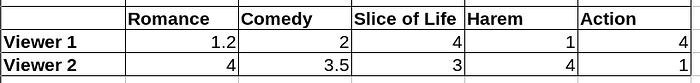
Viewer 1 prefers action and slice of life a lot more than other components, so, let’s compute the dot product of viewer 1 with all three anime. I’ll show the computation once manually below and you can similarly compute other dot products.

We take the two vectors Oregairu and Viewer 1 and multiply respective components together as seen in the snap above i.e. Multiply Romance Dimension of Oregairu with Romance Dimension of Viewer 1, Comedy dimension of Oregairu with Comedy dimension of Viewer 1 and so on. Finally aggregate these products together into a single value by summing.
Once we do this for all three anime we observe Viewer 1’s dot products are 29.2, 26 and 31.8 respectively. This means Viewer 1 likes Tokyo Ghoul the best which is indeed high on action.
Viewer 2 on the other hand is into romance and harem. His dot product with all three anime are 47.5, 35.5, 22.5 which means he would like Oregairu the most which is indeed a teenage love comedy with elements of harem!
After that otaku tangent, getting back to the topic at hand, we can see how representing viewers and anime as a vector can prove useful to determine a ranking of how a viewer would like all the anime or which users will like a particular anime and that’s a very valuable insight which streaming companies like Netflix are exploiting.
There’s also an additional component to both the viewer and the anime vectors which is called bias. It is a quantity used to represent unique information about that particular user or that particular anime respectively. So, if there’s a user who on an average rates all anime highly or there’s an anime which is a favourite across all/most viewers irrespective of their usual tastes, such information is captured by a term called bias. So, every viewer and every anime is represented in this structure using an n-dimensional vector and a bias term.
Collaborative Filtering in fastai2
fastai2 provides a sub-package fastai.collab that contains the functions to leverage for CF. After installing fastai2 on your system instructions here, you can follow along below.
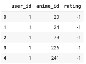
Mostly, data is stored or represented in this way. Although this is not a very intuitive way, it’s a pretty efficient way to store data. This is because most viewers haven’t seen most anime.
When such is the case, there will be a lot of zeros if we try to store it as a matrix of viewers v/s anime. Such matrices are called sparse matrices. There are efficient ways to store such matrices as well, however we would let it pass for the time being. Let’s focus on the task at hand now.
-1 here represents that the user has watched the anime but not rated it. This is a common scenario mostly because in reality, those who do watch the anime don’t necessarily provide a rating for the same. Having data always beats imputation but since we don’t have it now, we can either drop off the rows which have such a rating or we can impute the same. Imputation can be done in one of the two ways:
- Impute the rating with the mean rating for a user.
- Impute the rating with the mean rating for the anime.
Both of them have different interpretations. When we’re imputing based on the mean rating for a user, we are not paying heed to the relative characteristics of the anime in comparison with the other anime that the particular user has watched and similarly when we’re imputing with respect to the mean rating for the anime, we’re neglecting the relative rating of the user in question with respect to the other users. This might introduce a slight bias in our observations but we’ll be OK with it because of the tendencies of ratings to regress to the mean. If we choose to neglect those entries, we’ll end up scrapping a huge chunk of the data which would be detrimental to this analysis.
We will choose to impute the ratings with mean of anime rather than viewers here because we already have the mean rating for each anime provided to us in the anime.csv file. Here’s how the final distribution of ratings looks like
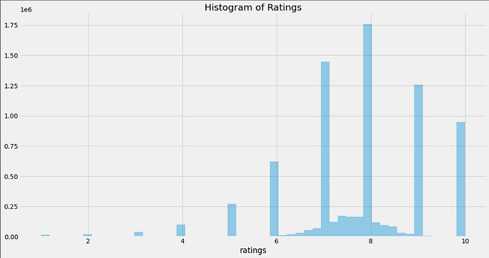
We can see that on an average, people tend be generous in providing ratings for anime. Most of them have provided a rating of 7 or higher and that leaves us with a left skewed distribution as can be seen above.
Now, we need to load the data in a specific format for feeding it to the neural network. The collabsubpackage of fastai contains a module called CollabDataLoaders which we can use in order to load the data.
Particularly since we’re loading the data from a pandas dataframe, we’ll be using the from_dffactory method to load the data.
So we create a DataLoader above. Since the names of columns could be application specific, we need to specify the names of user, item and ratings columns respectively.
The argument valid_pct stands for validation data percentage. Once we build a model, it’s actual sanctity is gauged by how well it performs on this data. Our model will be trained using 90% of the available data and tested on this 10% of validation data which it has never seen before. Only when our model performs well on both the training and validation sets, can we say that we’ve done a decent job.
With this dloader object, we can see what all it contains.

There are many anime in the dataset which have a very few almost no people rating for them. It makes sense to not include these anime because they’ll do more harm than good. This is because already there’s a huge sparsity in them which means there’ll be very very few updates with respect to them and hence very little learning. It naturally follows that the embeddings generated for such anime will be substandard and hence it doesn’t make any sense to save them.
Embedding Dot Bias Model
This model is a plain model just like we discussed in The basis section above. Both viewers and anime are represented as vectors and we get matrices for the same since there’s many viewers and many anime. Next, we do the dot product on them and compare them with our actual viewer ratings using the loss function Mean Squared Error which we aim to reduce. Eventually the model will become good at representing both the viewers and anime in this n-dimensional space.
Let’s create a simple Embedding Dot Bias model and train it.
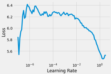
fastai2’s lr_find method of a learner object is really quite handy. We can use it in order to figure out which learning rates we should use for our training. It suggests the same as a tuple. The first value is minimum LR which would make sure some training occurs and the second one is that lr where there was the steepest fall in Loss. It’s good to select an lr that’s closest to the lr_min in suggested lr, prefarably a bit lower to be on the conservative end (personal observation).
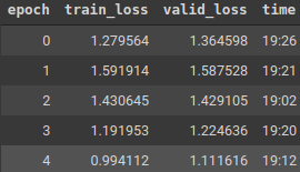
After training the model, we should see the loss reduce at each iteration. We can resort to early stopping if signs of overfitting are encountered (there could potentially be one here because in the fifth epoch, the training loss went up), so it’s good to keep the initial number of epochs small. Once you see the trend of train and validation losses, you can decide whether to further go ahead with the training or call it ends.
The Neural Network Model
On top of embedding dot-bias model we can build an MLP by adding fully connected layers for enhancing the complexity of models. Basically the user and movie vectors are concatenated and passed through a series of neural networks before taking the final dot product. Although in most of the cases, the former performs reasonably well, this neural network model also does work well in some other cases.
It’s a matter of performing trials and looking at the best performing network on evaluation of validation data that we can come to a conclusion on which model performs better. Let’s build a model using Neural Networks as well and test the performance on that.

The learning rate finder returns somewhat similar results however since we’ve increased the depth, we can see that the min_lr needed has went down. In my experience, when we increase the depth of a network, it is observed that the suggested lr_min decreases. We generally have to be more conservative with deeper networks because the convergence is more susceptible to the value of learning rate.
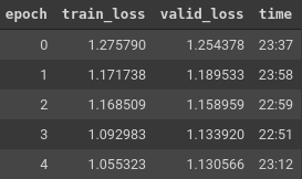
The training log is shown aside. It seems like adding the two FC layers at the end really doesn’t make a difference as the losses have furthermore increased as compared to the Embedding Dot Bias Model.
Model Interpretation & making Recommendations
Now that we have a model ready, let’s try to interpret it, use it and make some suggestions/recommendations.
Understanding Anime biases and weights/embeddings
Let’s try to understand the anime embeddings for the Embedding dot-bias model. First, let’s see what all layers are there in the model.
learn.model
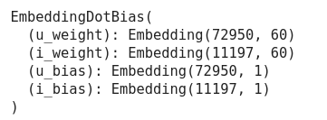
As seen above, there are two components for viewers and two for anime respectively, one being the vector and another one being the bias term respectively.
Let’s order the anime which by the most rated ones being the top ones (not rated highly but the most rated i.e. the viewers watched and rated the anime).

Let’s check the biases for these anime and compare them against the ratings for these anime. Similarly, let’s check the biases for the least rated (by count) anime and compare them against the ratings for the same. For the sake of understanding, let’s compare the top and bottom 5 out of these and see the results.
bias_rating_data.sort_values(by = ["Ratings"], ascending = False).head()
bias_rating_data.sort_values(by = ["Ratings"], ascending = True).head()

The anime which are rated highly generally have high biases. This is in line with the point above that the biases are high for anime which are generally liked by all viewers irrespective of their taste.
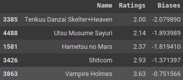
The anime which are rated lowly generally have very low biases. This is in line with the point above that the biases are small for anime which are mostly disliked by all viewers irrespective of their taste.
Next, as we discussed, the weights are nothing but vectors learned by the models. Let’s find out the weights of top 100 anime, apply a PCA on them to reduce their dimensions and then compare them visually on a 2-Dimensional plot. PCA is a dimensionality reduction technique used to compress vector/matrices and is commonly applied particularly when we have to visualise large dimensional data or if we face the Curse of Dimensionality problem in datasets with numerous features or columns.
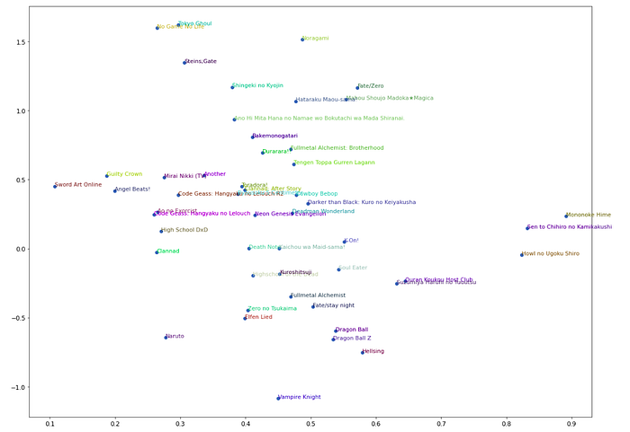
It could be seen that anime which are very high on action like Tokyo Ghoul and Attack on Titan are above the y=0.5 line and ones like Clannad, K-On, Ouran Host Club which are romance/slice-of-life anime are below that mark although there are a few exceptions. Also down to the right along the x-axis, romance and slice of life component seems to dominate more and more eg. Clannad After Story is to the right of Clannad and K-on, Ouran Host Club are furthermore to the right.
This is a compressed version of the data because of which there’s a lot of lost information that isn’t depicted here. We have reduced the dimensionality of the embedding vectors from 60 to 2 and yet we can see some structure to the data which is pretty awesome. Since humans are only bound to perceive the physical world in 3-Dimensions, we cannot visualise the 60-Dimensional Embedding space, hence this approximation.
Now that we have received the embeddings (True embeddings) for all anime, let’s compare the distances between Oregairu, Tokyo Ghoul and Hyouka.
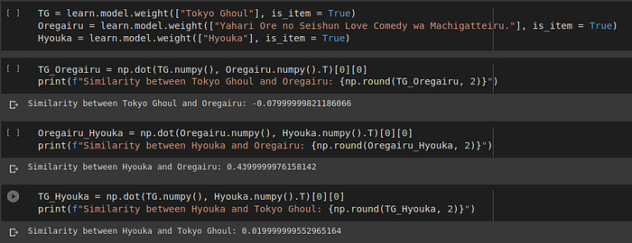
We can confirm that as we discussed earlier, Hyouka and Oregairu are indeed closer to each other since their dot product amongst the three is highest. Also both Hyouka and Oregairu are nearly equally far from Tokyo Ghoul by dot-product. This means the algorithm is doing a pretty decent job although it doesn’t really know which Genre the three anime in reality belong to.
Understanding User Weight/Embedding
In order to understand the user weights, we will randomly sample a user from our set and then in the remaining corpus, pick one user who is closest and one who is farthest from this randomly sampled user in terms of a specific distance metric known as cosine similarity.
Basically, we will take a dot product of that user, a user close to him and a user farthest from him in a span of the entire user corpus and then look at the respective anime to see the difference.
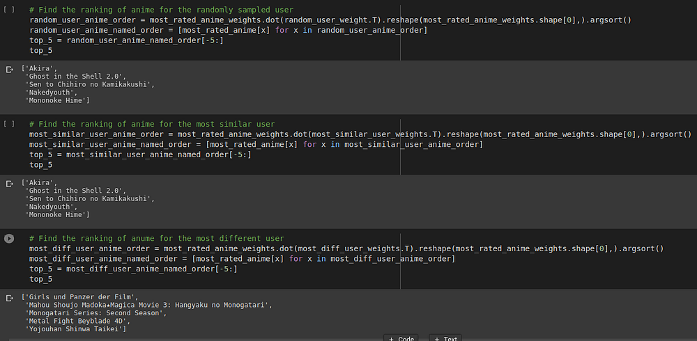
We see that our randomly sampled user likes anime which are high on action and fiction and involve some elements of drama/romance/slice of life. The most similar user also likes genres which are high on action and fiction.
It could be seen that the most similar user has almost all the anime picked which are same as the ones that the random guy liked and the most different ones have a higher degree of drama/slice of life involved in them.
A drawback of CF & potential solution
Now we looked at recommendations for users which are already present in database. If we have a new user coming in picture, we don’t have anything to suggest to him since he hasn’t rated any anime/movies.
This is commonly referred to as the Cold Start Problem.
To work around this problem, the new user is asked a few questions which pertain to his likes and dislikes on the anime present in our catalogue. This makes the system recommend a few anime and as the user engages more frequently with the platform and gives feedback, the recommendations become more and more refined to suit the tastes and likes of the viewer.
Collaborative Filtering or Recommender Systems are here to stay and help viewers/users/consumers/subscribers get content suitable to their likes and tastes. Hope this post helped you to get a quick overview of the same and happy learning! If you want to dive further deep, I have suggested some articles in the Reference section.