
Multi-label Classification with Spreadsheets
Written: 18 Aug 2021 by Vinayak Nayak 🏷 ["fastbook", "deep learning"]Table of Contents
Introduction
Many a time we come across images which have multiple objects of interest. For instance, in the following image we can see that we have both a chair and a tvmonitor.

To solve the above problem, we need to be able to detect multiple classes/labels in a given image. This is what multi-label classification is. Given an image, categorize it into more than one class/label/category.
Since fastai is a very convenient wrapper around Pytorch, there’s very little that we will have to change from the perspective of code but the logic behind solving this problem will be somewhat different. We cannot just use our regular softmax activation with cross-entropy loss function; also the evaluation bit here is much more involved than that of a single-label classification problem. We shall discuss every bit in detail in the following sections. Let’s first begin with the dataset.
Dataset
We will be using the PASCAL_2007 dataset for this task. This is a dataset which contains 20 labels in all and mind the fact that one image can have multiple labels!
Simply use fastai’s untar_data to download the dataset to your disk. It will be stored in a special directory called .fastai at your home/root location
from fastai.vision.all import *
path = untar_data(URLs.PASCAL_2007)
If we look at the stats from a label POV for our train dataset, we obtain the following.

From the above figure we can see that person is a highly recurring category in the train dataset and other categories are more or less equally represented. So, we have an imbalance in our dataset.
Another interesting thing to note is that the sum of label counts is not the same as number of datapoints. In single label this used to be true because every image had one and only one label but in case of a multi-label classifier, since each datapoint is not bound to have only one object, it is worth noting that there can be more labels than number of images. This will lead us to change our strategy for building classifiers as against single-label classification.
In this dataset, we’re given the labels in the form of a dataframe and not in a folder structure same as Imagenet. So we’ll have to read each entry from the dataframe and define getter methods to retrieve the values of input and output. Also, the split is defined using a column in the dataframe called is_valid. We shall define a custom function that provides the splits i.e. indices of the train and validation set separately for all the points in our dataset.
In code, this looks as follows
# Define the getter for independent variable
def get_x(row): return path/'train'/row['fname']

# Define the getter for dependent variable
def get_y(row): return row['labels'].split(" ")

# Define how to split the data into train and validation
def splitter(df):
    valid_idxs = df[(df.is_valid == True)].index.tolist()
    train_idxs = df[(df.is_valid == False)].index.tolist()
    return (train_idxs, valid_idxs)
Now, we can define a dataloader once we have the proper getters for the three main tasks i.e. getting dependent & independent variable and how to split them into train and validation files. Unlike single label classification tasks, for this task, we will have to use the MultiCategoryBlock in order to read our dependent variables as one-hot encoded vectors. The rest of the loading remains the same. We can load the data as follows
# Define a multicategory block with presizing
dblock = DataBlock(blocks=(ImageBlock, MultiCategoryBlock),
                   splitter=splitter,
                   get_x=get_x,
                   get_y=get_y,
                   item_tfms = RandomResizedCrop(460, min_scale=0.35),
                   batch_tfms=[*aug_transforms(size=224, min_scale=0.75),
                               Normalize.from_stats(*imagenet_stats)]
                  )

# Define your dataloader
dls = dblock.dataloaders(df, bs = 32)
- Our independent variable is an Image hence
ImageBlockas input followed by aMultiCategoryBlockfor one-hot encoding and loading the dependent variable. - Our splitter is defined above which takes the
is_validcolumn from our dataframe and based on that boolean variable separates train and validation entries - The
get_xfunction reads the columnfnamethe filename and appends the base path to the file for loading - The
get_yfunction reads the columnlabelsfrom the dataframe and since our labels are space separated, it splits the labels string by using the space delimiter. item_tfmsandbatch_tfms: We use thepresizingtrick from fastai to avoid lossy image cropping (like padded borders etc.) and standard augmentation methods followed by a Normalization using theimagenet_statsas we would be using a pretrainedresnet50for this classification task.
Now, if we look at an example of a batch, we can observe the following. Look at how we have multiple labels in images from these examples.

Model And Activation Function
Although using the fastai API to define the model and loss is pretty straightforward, we should pause for a bit and look at the Loss Function and model, especially the loss function in detail.
There are several changes which we are going to do toward the model head. We are not going to use softmax as before but sigmoid activation.
\[Softmax \ Activation \ {i} = \frac{e^{z_i}}{\Sigma_{j=1}^{N}e^{z_j}}\]What softmax does is it will transform the logits coming from the final classification linear layer to always sum up to 1. What this means for multi-label classification is that we would incur high losses when we encounter examples having multiple labels. Consider the following scenario for example

We see that for this hypothetical example, the datapoint actually belongs to class 1 and 4 but the best our softmax can do is push the probability scores of these two classes to 0.5 and that of the remaining two to be 0 but no better than this. This is because probabilities must always sum to 1. Imagine if it were a three class example,then the best softmax could do is push the three probability scores to 0.33 and that of the remaining 1 to 0.
Now, let’s look at Sigmoid Activation.
\[Sigmoid \ Activation \ {i} = \frac{1}{ 1 + e^{-z_i}}\]Now, we see that the activation function doesn’t care what the other labels are. It is only focussed on the logit for the label in question, unlike softmax.
The logits are all decoupled and do not impact amongst themselves as against softmax.
This is why in the figure above you can see that the Sigmoid activation probabilities for classes 1 and 3 can climb high to approach 1 and the other two can approach 0 independently.
Now, you can appreciate better why we cannot use the softmax activation function but need a separate sigmoid activation function for this problem.
Since we have changed the activation function, we ought to reconsider our choice for the loss function.
For single label classification, we use the cross entropy loss function defined as follows
\[Cross \ Entropy = - \Sigma_{i=1}^{N} t_i \times log(p_i)\]where ti is the true value and pi is the probability predicted for a label
If we continue applying this loss function to our sigmoid activated outputs, we’re in trouble. We will not then be penalizing anything where the ground truth label is 0. For the same example above, if we compute the CE loss we see the picture as follows

On the other hand, Binary Cross Entropy is defined as follows
\[Binary \ Cross \ Entropy = - \Sigma_{i=1}^{N} (t_i \times log(p_i) + (1 - t_i) \times log(1 - p_i))\]where ti is the true value and pi is the probability predicted for a label
Now this is really interesting. It makes sure that whatever the label (0/1) some loss will always come to penalize the model for bad predictions. It will never be zero. Where ground truth is 1, the loss will be -log(p) and where it’s 0, the loss would be log(1-p). This would be very useful for the model to individually penalize the model via the different neurons in the classifier head for their mispredictions.
In the image above, we can see how even when the ground truth label is 0, we are getting finite loss values for those neurons as well as against plain cross-entropy loss employed in single-label classification.
For model, we can still continue using our imagenet pretrained backbones and start with transfer learning.
Why the same model even if the task is different -Single Label as opposed to Multi label Classification?
Although in the end we have to predict multiple labels per output, we still can make use of the same filters which were pretrained to identify humans, animals, objects etc. that were a part of the big imagenet dataset. The pretrained backbone which has intelligently learned these 1000 classes has filters which could detect faces of humans, fur of cats, tails of dogs etc. and similar classes are also present in the PASCAL_2007 dataset. Hence it makes sense to start with this as the anchor point to leverage what we already have!
So, we are now in a position to define a fastai learner to do the training. It is as follows:
learn = cnn_learner(dls, resnet50, metrics=partial(accuracy_multi, thresh=0.5))
Here we have changed the metrics to use accuracy_multi instead of plain old accuracy. We will discuss this in detail in model evaluation but apart from that we haven’t changed anything from when we were doing Single label classification, or have we?
Under the hood, fastai selects BCE loss because we have specified in the dls, our dependent variable is a MultiCategoryBlock. We can explicitly specify it but we need to be aware of it at least.
Then the training and lr_find and other things remain the same as shown in the following snip.

Model Evaluation
This is the most important part as this is considerably different for multi-label classification.
Firstly, what is accuracy_multi?
In case of multi-label classification, our targets are one-hot encoded. Also the outputs that we get are of the same shape as the targets but they’re logits. So we apply sigmoid activation on those and get probabilities.
In single label classification, we were comparing only one label for a datapoint and if it matches, our result is accurate otherwise it isn’t. However, for multi-label classification, for every datapoint, we predict a vector and the output is also a vector. So we need to compare these vectors instead of a single scalar for every datapoint. Since we have to compare multiple values, and then take an average across these comparisons; hence the name accuracy_multi. The following table will summarize this better.

Predictions -> Probabilities to Presence/Absence
As we saw in the example above, we assumed predictions as a binary field but the neural network by itself does not give us a discrete value for each class/label. It gives us an array of floats which we need to convert into a probability distribution and subsequently into a discrete value representing the presence/absence of a class/label.
First part is simple and we have covered it i.e. going from logits that are output from the neural network to a probability distribution only involves applying a sigmoid activation to the probability values for the respective classes.
For the next part i.e. converting probability into a discrete value; we have to do thresholding. What this means is we select a probability value and we use that as a pivot to convert the continuous probabilities into discrete distributions. The following example will explain this phenomenon better.

As seen in the image, we first take the network outputs and apply sigmoid activation which gives us the probability. Next, we arbitrarily pick 5 thresholds [0.1, 0.3, 0.5, 0.7, 0.9]. Now, what we do is compare these probabilities against the thresholds. When probability > threshold we mark it as True and False otherwise. Then taking an average across the predictions gives us the accuracy for that datapoint.
In single label classification, the accuracy for a single datapoint can be either 0 or 1 whereas in multi-label it could be a continuous value between 0 and 1 inclusive of the two.
Now, since we’re talking about thresholds it becomes important for us during evaluation to figure out what threshold is the best. Also, currently we’re using the same threhsold for all the classes/labels. We can tune the threshold over each class separately to come up with a best score for each class and then use those thresholds to get the multi-accuracy across the entire dataset. Let’s see how to do that.
Global thresholding
What we did above could be in some sense called Global Thresholding where we used a threshold for all the classes, compared the accuracy for each datapoint, came up with a plot which compares accuracy against the threshold and pick the one which gives the best accuracy.
Here’s how we could do it in code
def threshold(preds, targets):
    # Define 100 thresholds equally spaced from 0 to 1
    thresholds = np.arange(0, 1, 0.01)

    # Create a mapping from threshold to accuracies
    thresholdAccuracyMapping = {}
    for thresh in thresholds:
        thresholdAccuracyMapping[thresh] = accuracy_multi(preds, targets, thresh = thresh, sigmoid = False).item()

    # Create a dataframe out of the above mapping
    df = pd.DataFrame(thresholdAccuracyMapping, index = ["Accuracy"]).T.reset_index()
    df.columns = ["Threshold", "Accuracy"]

    # Make a plot
    fig, ax = plt.subplots(1, 1, figsize = (6, 4))
    sns.lineplot(data = df, x = "Threshold", y = "Accuracy", ax = ax)
    fig.suptitle("Accuracy at different thresholds", fontsize = 24)
    fig.tight_layout();

    # Plot the best threshold
    bestThreshold = df[df.Accuracy == df.Accuracy.max()]
    bestThr = bestThreshold.Threshold.item()
    bestAcc = bestThreshold.Accuracy.item()
    ax.scatter(bestThr, bestAcc, c = "red");

    # Return the best Threshold
    return (bestThr, bestAcc)

This function above gives us the best accuracy point and the threshold at which it occurred which could be simply saved as a artefact with the model and during inference, when we wanna get predictions for individual labels, we can compare their probabilities against this threshold and get the discrete results to denote presence/absence of a class.
However, we can do better.
Class/Label level thresholding
In practise, accuracy is not always the best evaluation metric. For eg. in a world where there’s only let’s hypothetically say 1% people who are rich, predicting every person to be poor no matter what will make you 99% accurate, but is that really good?
No, right? When you create a classifier where there’s heavy class imbalance, you want your performance to be good across all classes and not just one or two classes which are very highly dominant in your dataset. Accuracy cannot tell us such information. Here, having other metrics like Precision, Recall/TPR, FPR, f1-score etc. become very useful. This post is not meant to deep-dive into these metrics but let’s take a cursory glance at them and I will provide good resources at the end to delve deep into each one of those.
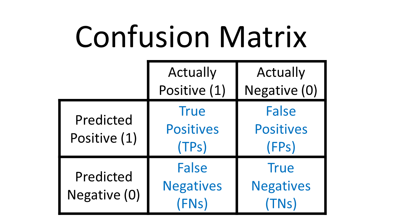
Precision: This quantity basically tells you of all those examples which are predicted to be of a certain type, how many were actually of that type. If we look at the confusion matrix above, we can define Precision as
Recall/TPR: This quantity basically specifies how many examples of a particular category were properly identified by the classifier. It is also called asTrue Positive Rateor TPR for short. It is given by
f1-score: When we’re defining a classifier, we want the two to be as high as possible and ideally to be 1 but they’re kind of both inversely related to one another. Hence we define a metric which finds the point where they’re both best balanced. This is the f1-score which is in principle a harmonic mean between the recall and precision defined as follows
FPR: False positive rate is the number of negative examples which are misclassified. It is given by
The evaluation of a classifier can be done on several grounds. For some accuracy could still be the gold standard of evaluation; for some others, f1-score might be an important figure to ensure the classifier performance across multiple categories. In many cases, the ROC or receiver operating characteristics plot could be used to figure out the classifier performance. We will evaluate our model using all the three techniques to get the best performing model given a specific criterion.
A graph of ROC for bus category from the PASCAL_2007 datset on which we trained our model is as follows

On the X-axis we have FPR and on the Y-axis we have Recall/TPR. We need to identify the point where the TPR is as high as possible without the FPR increasing. We can figure this out by finding the point which is closest to (0, 1) point i.e. where FPR is 0 and TPR is 1. This is shown in the curve with the red dot. For a perfect classifier, we should have a unit-rectangle kind of a graph but practically the distributions of the two classes are never completely distinguishable in most cases.
The complete code to do this will become very large but it is available on github which I have attached in the references section. I will sketch out the pseudo-code for doing this local thresholding and then final aggregation of the predictions.
1. Get the predictions & targets from the fastai learner
2. Separate out the predictions and targets for each and every label. The fastai predictions would be of shape `N_EXAMPLES x N_CLASSES`, so break them into N_CLASSES vectors of length `N_EXAMPLES` each. Similarly do this with the targets.
3. Select a range of thresholds and evaluate the metrics precision, recall, fpr, f1-score for all the examples of each class/label and construct the ROC-AUC Curve.
4. Select the closest point, best accuracy and best f1-score points amongst all those points over which you varied the threshold. Record the threshold for each of those points where you obtain the best of these metrics.
5. Using the recorded thresholds for each class obtained from 4, convert the probability distribution into a discrete one and find the overall accuracy of the multi-label classifier.
If we were to make a comparison, individual class/label’s threshold tuning with the bestAccuracy strategy for each class gave us slight jump in accuracy over the global thresholding which also gave us a slight jump as against the default threshold of 0.5 which is commonly used in all classification problems.

Conclusion
- Multi-label classifier (MLC) can tag a given datapoint with multiple classes/labels.
- The activation used in MLC is
sigmoidnotsoftmax. - Loss function used for MLC is
BinaryCrossEntropynotCrossEntropy. - A good threshold can make a significant difference in getting better/worse accuracy for an MLC.
- During model evaluation, accuracy may not be the gold standard and metrics such as recall/precision/f1-score will be useful especially when there’s class imbalance when training the model.
I hope you enjoyed reading through this blog-post! I would be glad to connect with you on Twitter. If you have any comments/suggestions/thoughts, feel free to comment below or reach out to me on Twitter.
If you liked what you read, feel free to check out my other posts here..