
Time series forecasting of Indian Stocks using LSTMs in PyTorch
Written: 26 Oct 2020 by Vinayak Nayak 🏷 ["deep learning", "visualization"]In this post, we learn how we can predict the trajectory of stocks interactively with a sequence model. The table of contents of this post is as follows

- Introduction
- Extracting equities historical data using nsepy
- Curating Data to pass it to an LSTM model
- Defining the LSTM model architecture
- Training the model
- Making predictions on unseen data
- Conclusion
- References
Introduction
Time series data has been around for quite a while and many people have studied them and came up with ways to analyze the data to find meaningful insights and subsequently use it to make reliable predictions as to how the series will progress in the future. Stock market investors have leveraged this information to gauge the performance of stocks to make smart investment decisions. Traditional time series algorithms like ARIMA, SARIMA, Holt-Winter’s method etc. do a good job in modelling a time series; however in the recent times, with advent of deep learning, recurrent neural networks have grown in popularity for modelling sequence data.
Since time series is basically a sequence, RNNs (LSTMs in particular) have proven useful to model them. In this post, we will be building a dashboard using streamlit for analyzing stocks from the Indian Stock Markets using LSTMs in PyTorch. Stocks data will be scraped using nsepy — an open-source python library developed & maintained by Swapnil Jariwala . Without much further ado, let’s dive straight into it.
Extracting equities historical data using nsepy
The Indian stock market (equities) consists of 1655 listed equities as of now, this data could be obtained from here. With the help of the ticker column in the csv file extracted from this site, we can use nsepy to get historical information for any listed stock using the predefined get_history function in the package. It could be done as follows.
One has to simply provide the stock ticker info, the date from which and upto which they want the historical data for that ticker. The extracted data is obtained as a pandas dataframe and we’re interested in the date and close columns from the same for the sake of our analysis.
This function by default returns the equities historical data, you could also obtain options data for the respective stock by passing in the option type, strike price and contract expiration date. Or you can pass the futures argument to true and pass the expiry date to get the futures data as well.
The nsepy library is a convenient library with well written functions helpful for anyone who wants to perform analysis on stock data. More about it here.
Curating Data to pass it to an LSTM model
Once we get the data from the website, it would look something like this.
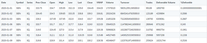
We will be working with the date and close fields from the above table i.e. we will build an LSTM model which predicts given the close value of previous n days, what would the close value be on the current day. The number of steps upto which we look in the past is commonly known as the number of lags or lags simply. We will keep it as an input from the user so that they can experiment with it and see for themselves.
There is a series of steps that you need to follow for bringing this data in a format which could be loaded in the pytorch model. Here’s listing them down chronologically.
-
Extract the columns of interest from the dataframe shown above. (Close and Date columns).
-
Shift the dataframe down by number of lags times and remove the first number of lags rows. This will give us input output pairs in a columnar format. This could then be converted into a list of tuples for input and a list of floats for the output value of the stock price. The logic for this is defined in the function below.
- For feeding data to a model in pytorch we need to create a dataloader which generates batches of inputs and outputs. Pytorch provides support to build our own custom dataclass and wrap a dataloader over it in order to feed data to the model as we wish. So, we will extend the Dataset class and define our own class as follow
- The pivotal function above is the get item function which feeds inputs and outputs. We wrap them into torch tensors from the lists which they currently are because pytorch models only accept data which has datatype of a pytorch tensor. Since the prices are decimal numbers, we wrap the data meticulously into float tensors.
In any Machine Learning algorithm, it is important to validate our dataset on previously unseen data to make sure the model that we’ve built is not memorizing the training data which would lead us to falsely believe that our model is performing extremely well when in fact it isn’t (overfitting).
-
To address the above fact, we perform a train-validation split with 70% of the data in train set and 30% data in validation set.
-
One more crucial aspect which is very important particularly from a deep learning perspective is to avoid covariate shift.
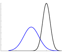
When we have more than one feature in a predictive model, it is possible or rather mostly the case that they have different distributions and are on completely different scales. Because of this, the cost function that the neural network tries to optimize becomes more difficult as the loss landscape tends to be unevenly spread. If instead we bring the two distributions to a homogeneous scale, the error landscape becomes even and that helps the neural network optimize the cost function much better. One method to accomplish this is standardization of the input data which in principle, converts all the input parameters to have a mean of 0 and standard deviation of 1. Internally in the different layers of the network, batch normalization is used to avoid covariate shift problems. The following function therefore standardizes the data based on input i.e. train distribution.
- After having split the data into train and validation datasets and subsequently standardized the same, we will create pytorch dataloaders in order to load the data and feed it to the pytorch model later on.
Now that we have all the data ready in the necessary format, we shall switch gears to define an LSTM model for predicting stock prices.
Defining the LSTM model architecture
LSTM or short for Long-Short-Term-Memory is a Recurrent Neural Network which is used for modelling problems involving sequences. There are several input-output usecases possible for sequence problems like one to one (word translation), one to many (image caption generation), many to many (laguage translation); but our case is many to one i.e. given a list of inputs, we’re predicting one output.
For sequences of reasonably short lengths (less than 15–20 units per record), LSTMs do a wonderful job of decoding the correlations and capturing them to build a robust model but because of vanishing gradient problems, they can’t capture long term correlations; we will revisit this later when we review the model predictions.
For now, let’s focus on creating an LSTM pytorch model.
We shall now go through all of the above code step by step.
As we can see aside, our model consists of an LSTM layer and two fully connected linear layers.
LSTM layer needs a three dimensional input of the form
(seq_len, batch, input_size)
Batch size is a training hyperparameter which can be set at the time of training, seq_len and input size are two parameters which we need to be aware of from our dataloader. Since we’re going to look at n_lags historical stock prices, our seq_len is 3 and we’re only looking at one feature which is stock price so our input_features are only 1.
Also our hidden and cell states are defined to be all zeros (They could also be defined as random numbers at the start of training).
The forward method contains the logic for the forward propagation through the network. We pass the input through an LSTM layer, then through a fully connected layer; this is followed by a batch normalization layer to prevent internal covariate shift and a non-linear ReLU activation layer. Finally we pass it through the output estimator layer which gives us the predicted stock price.
The predict method just implements the forward pass but by switching off the gradient tracking functionality as we only want the prediction and don’t want to do any back-propagation.
This is just a basic architecture which could be tweaked and modified as per the needs of the problem. Feel free to add or subtract fully connected layers, change the hidden dimensions and the number of hidden layers inside the LSTM layer and regularise using more dropout layers as you deem fit.
Training the model
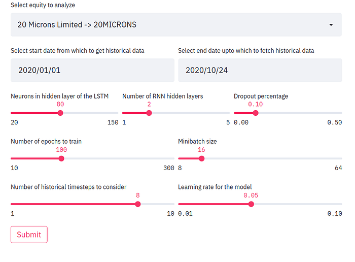
We have now reached the crucial part of training the model. We will have to define a lot of hyperparameters before we start the training and here, we shall use streamlit to allow the user to interactively define the same. Some of these are the batch size, learning rate, the optimizer, number of hidden layers, neurons in the hidden layer etc.
Once these are selected, you can hit the submit button to see the model train in action. Here’s one such example in action.
We loop over the data in the training generator for n_epochs number of times to train the model.
In every epoch,
- We loop over the data in training generator that we created above and use the Mean Squared Error (MSE Loss function) in order to optimize the model to predict the stock prices appropriately.
- We loop over the validation generator to evaluate the performance of model trained so far and calculate the loss for the same.
- We store the losses for displaying them to the user later on and for internal auditing purposes.
- After every forward pass, loss is calculated, it’s backpropagated through the network by the optimizer when it takes a step in the direction of the minima. We must prudently overwrite the gradients to zero before a new batch’s loss are backpropagated and then calculate the average loss for that batch. In brief, this is the training loop that most pytorch networks follow with a few changes here and there.
Making predictions on unseen data
Once we have a trained model ready, we can now perform predictions on previously unseen data that we had set aside as validation data at the beginning of training. We shall do that and plot it to analyze the performance of that model.
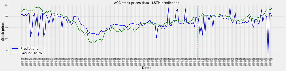
This is the result of a model which had data corresponding to ACC stock from 1st January 2020 to 15th October 2020 with a lag of 8, hidden layers of 100, trained for 100 epochs with 2 hidden LSTM layers. We can see that the model has picked up the overall trend of the stock prices but it’s highly unstable i.e. it overestimates changes in prices by a substantially big margin. Also if you’re keen you can observe that in some cases, the predictions lag the actual event i.e. if there’s a sudden jump today, the predictions will show that jump tomorrow and so on.
The blue line separates the training and validation datasets; to the left of the line is train data along with it’s predictions and to the right of the line is the validation data with it’s respective predictions. We can see that the validation and train predictions are pretty much similar in behaviour which is a good sign since it’s consistent in the prediction pattern across both seen and unseen data.
This is something that needs extensive hyperparameter tuning and one can go about it in a brute force/organized manner to look which configuration of parameters work best for which stock ticker.
That’s the reason why I built an interactive dashboard using streamlit. They offer great support to build interactive dashboards using sliders, dropdowns etc.; All without having to know any HTML, CSS and JavaScript which is pretty awesome. Check out their medium publication here for more amazing visualization stuff.
Conclusion
So, that’s it for this post. In this post, we learnt to
- Extract stock ticker information pertaining to Indian equities using nsepy.
- Create an LSTM in pytorch and use it to build a basic forecasting model with one variable.
- Experiment with the hyperparameters of the model to tune it to become better in an interactive fashion using streamlit.
Hope you liked the post and learned something from this. If you wanna dive deeper, please see the references section for more involved articles on the topics covered in this post. Also all the code for this post is available in references section as well.