
Advanced operations with Numpy Arrays
Written: 27 Aug 2020 by Vinayak Nayak 🏷 ["basics"]In my previous post, I talk about Reduction Operations in Numpy Arrays. You may read through it before you move on to the more Advanced Operations below.
The topics covered in this post are as follows:
- Introduction
- The Dot Product
- Singular Value Decomposition
- Inverse of a Matrix
Introduction
Numpy consists of a subpackage called linalg which has functions particularly pertaining to linear algebra which is an integral part in the working of many DL and ML algorithms. We will discuss several concepts about these operations along with their numpy implementation which will inevitably become a part of your Data Science toolkit. We will be covering three of the most important operations that can be carried out with numpy arrays which are heavily used in DL and ML applications such as Natural Language Processing, Image Retrieval tasks and Customer Recommendation tasks. Without any further delay, let’s get started!
The Dot Product
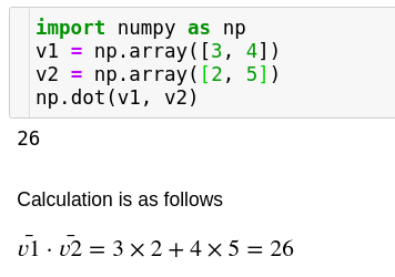
In vector algebra, the dot product represnts a scalar quantity obtained by sum aggregating the product of vectors along the n-dimensional space respectively. In linear algebra, dot product is typically used for finding out if two vectors are perpendicular to each other or to find out the magnitude of a single vector or to find out the projection of a vector along another vector.
In Data Science, the dot product is typically used to find out the similarity or distance between two or more vectors in some high dimensional space. When we perform nearest neighbour search this is what we typically use. The similarity found out using dot product is called cosine similarity because the dot product theoretically is given by the expression
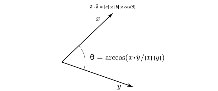
The smaller the angle between the two vectors, more closely aligned the two vectors are since the cosine of an angle is high when the angle itself is small/low.
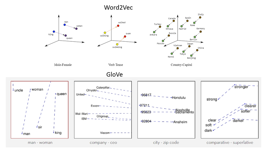
In Natural Language Processing applications, the words are individually represented as vectors or embeddings of different lengths (50, 100, 200, 300, 512 etc.) Dot products are used to identify word similarity and word relationships which emerge out of words being used in similar contexts; such as country-capital pairs, or male-female pairs and so on.
In applications such as visual search, the images are converted into a single dimensional vector which are compared on the basis of dot product as discussed above to retrieve similar looking items or images.

Singular Value Decomposition
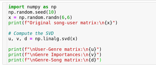
This is a concept very commonly used in recommendation systems. Basically, it is used to extract topics or genres or gists of information from a consumer/user/record v/s product/movie/song/feature matrix respectively. (We’ll use user and song respectively in our example).
The topics extracted by SVD are abstract and may not really be in the scope of humans to understand. But generally it’s observed that most of the times it’s identifiable what the topic can broadly be a manifestation of. For example, consider we have constructed a matrix which has names of novels as rows and individual words in the novel as columns where each value represents the relevance of that word in a particular novel (the underlying method is called tf-idf which we won’t dig deep into now). This matrix can be decomposed into three matrices which can help us understand the vectors in more detail.
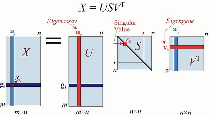
The first one is the user-topic matrix, the second one is the topic importance matrix(this is always a diagonal matrix where the diagonal elements are representative of importance of the respctive topic) and the third matrix is the topic song matrix. Once we have these matrices, we can utilize this information to create buckets of users to suggest music from respective topics which they like to hear. Whereas the terms users and songs here are for the sake of better understanding, it could very possibly be novels-words, users-movies etc.
By default the number of topics is the same as the number of songs/words in the above case but that doesn’t serve the purpose because every song or word will be a genre/topic of it’s own that way; so in practise, there’s another version of SVD that we use called truncated SVD in which the number of topics is restricted in number. This gives us a workable number of topics that are meaningful for recommendations.
Numpy doesn’t offer a function to perform truncated SVD. We have to use another library called scikit-learn to do the same; don’t bother much about it, I will cover it in detail a future post. However it’s important to note that truncated SVD is more commonly used because it acts like a tool which can extract meaning from these numbers while compressing the information substantially to a useful state.
If you’re really interested to dig deeper into the topic, I would recommend you read this post which covers svd in great depth with all the math worked out beautifully.
Inverse of a matrix
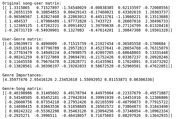
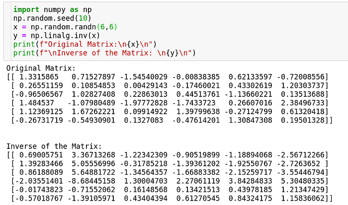
The inverse of a matrix is a matrix such that when it’s multiplied with the matrix itself, we obtain an identity matrix. Now, why is such a matrix useful?
For a long time, solving systems of linear equations in order to find out unknown variables has been prevalent which in my honest opinion could be considered the origins of data science. Because understanding natural phenomenon, quantifying them into constraints and expressing them as a system of linear equations to find out the values of unknown variables using numerical methods involved dealing with observational data and is still used significantly in the computational fields.
That’s why the inverse of a matrix becomes an important quantity when we solve these equations. The general formulation of the problem is
\[AX = B #therefore X = A^{-1}B\]The first quantity in RHS of the second equation is called inverse of matrix A. Numpy offers an eponymous function to compute the inverse of a matrix.
The first quantity in RHS of the second equation is called inverse of matrix A. Numpy offers an eponymous function to compute the inverse of a matrix.
Well, matrices is an expansive chapter and there’s no end to it. These three operations in the world of data science are the most commonly used and make it to being an invaluable tool in your data science toolbox. One other method known as PCA is very similar to SVD, apart from this, there might be other tools like cross-product/vector-product etc. which are not very commonly used in data science, so we’ll save those for a later day.
The code snippets above can be viewed on my github in this repository Numpy Explained.
Thanks for reading through this entire series of getting to know about Numpy Arrays and hope these tools work in your favour when working on your data science solutions!