Special Arrays in Numpy

If you’re new to arrays in numpy, I would recommend you first have a look at my previous post here to get accustomed with arrays in numpy and then continue forward.

Topics covered in this post at a glance are as follows.

• The All Zeros Array
• The All Ones Array
• The Identity Matrix
• The Diagonal Matrix
• The Linearly Spaced Array
• The Log Spaced Array
• Random Arrays
  • Reproducibility in Randomness
  • Random Normal Array
  • Random Uniform Array

Numpy has a huge number of functions/methods and some of them can be effectively used in order to conveniently create arrays which are frequently encountered in Machine Learning/Deep Learning problems. So, without any further ado, let’s dive straight into discussing these special arrays, how to create them and where they’re useful. Please note that I will be using the terms array and matrix interchangeably in the subsequent part of the post.

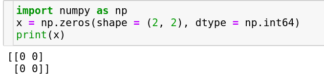
The all zeros array

Just as the name suggests, this array contains nothing but zeros. It could be of any size/shape which the user provides and also the datatype can be specified by the user optionally.

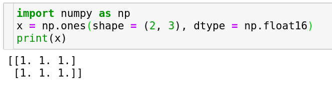
The all ones array

This is an array where each and every element is one. Similar to the all-zeros array, this could be built using the np.ones function by specifying the shape and optionally the datatype of the elements in the array.

Both the all-ones and all-zeros arrays can be used particularly for setting flags, for one-hot encoding label/target variable in Machine Learning applications, as a placeholder for filling in the values based on some set of operations etc.

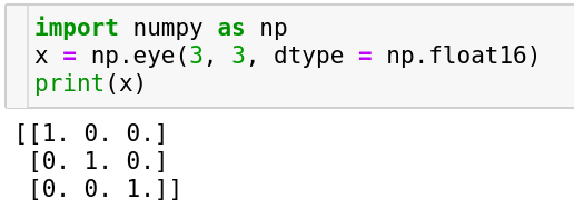
The Identity Matrix

In the world of matrices, the identity matrix plays a big role. It is a matrix having ones on the diagonal and zeros elsewhere. It’s handy in computing inverses, in finding the identity-mapping representation in resnets and in quite a lot of places.

It is typically encountered in a square form but not necessarily. It could be a rectangular matrix as long as all the diagonal elements are 1 (diagonal elements are the ones which are accessed using same index across all the dimensions). In numpy the np.eye function is useful to create an identity matrix and it can be used similar to the ones and zeros function by specifying the dimensions and dtype (optionally) of the array respectively. Please note that here dimensions are specified separately unlike as a tuple in the earlier examples.

The Diagonal Matrix

A matrix which has all zeros across the non-diagonal elements is called as a diagonal matrix. Conversely, it’s only the diagonals which are permitted to have non-zero elements in this matrix. Since it’s quite common to encounter diagonal matrices in techniques like Singular Value Decomposition, Eigen Value computation and stuff which can possibly be utilized in Machine Learning for building recommendation systems, the good people at numpy have provided us with a function which can convert a diagonal matrix into a vector of diagonal elements and vice versa. Let’s see how.

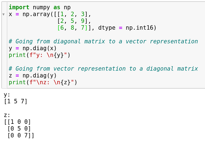
As we can see in the first turn, a 3 x 3 array was converted into a 1 x 3 array which only comprises of the diagonal elements of the parent 3 x 3 array. Conversely in the second step, a 1 x 3 array was converted into a 3 x 3 array. Please note that we can use np.diag to dig out the diagonal elements irrespective of whether the source matrix is a diagonal matrix.

The linearly spaced array

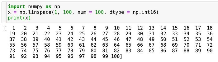
Many a time we want to create arrays which run incrementally from a particular start value to a stop value in many computer-science as well as machine-learning applications. Loops would be one example of a linearly spaced array which are supposed to run for a particular number of steps.

Numpy provides a function to do just that. All you have to do is specify the start, the end and how many items you want in between.

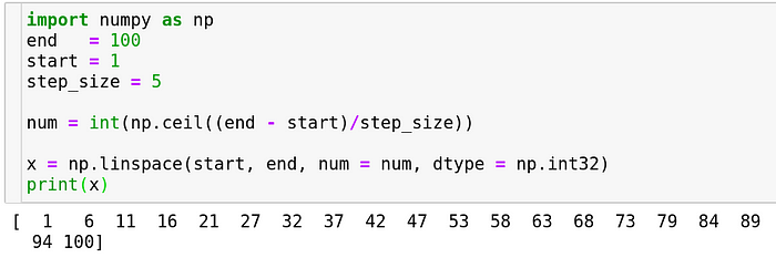
On the other hand, if you knew the step size and the start and end you could use the same function as follows. Note that in order to accommodate the end integer, the function will do some adjustments on it’s own, like how it didn’t consider 99 because after 99, we would have 104 which is out of the range and we want 100 i.e. the end number to be in the range.

This is used typically for looping over things, looping over every odd/even/spaced over some interval etc. It comes in handy during pre-processing data stage of an ML solution cycle.

The logspaced array

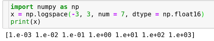
Just as we have the linearly spaced array, we can also have arrays that are spaced on a log scale. This is particularly useful while dealing with quantities that vary on a logarithmic scale. Just like we specified for linspace, logspace takes in the start and end quantities and number of elements that need to be in between the two of them and optionally a datatype which each element of that array should be in.

We can make use of this feature when we are doing hyperparameter tuning for learning rate in deep neural networks, or when we have to deal with features that grow in a geometric progression and so on.

Random Arrays

When doing machine learning which involves statistics to a considerable extent, the need for random numbers arises inevitably. Although we cannot generate random numbers, we can simulate the production of random numbers using a pseudo-random number generator and numpy gives us one of those in the subpackage random. We will cover some aspects of this subpackage pertaining to arrays here.

Reproducibility in randomness

Since we’re simulating randomness, we can make sure that the randomness that I generate resembles the randomness that you generate when you run the code that’s provided here (Well, that’s why it’s pseudo-random and not random). In order to do so, you just have to set a seed. You can do it as follows

import numpy as np
np.random.seed(10)

The argument in the above function could be any integer. As long as it’s the same and the numpy and python versions are the same, running any of the following commands after setting the seed will ensure that you get the same random numbers.

Random normal array

A normal distribution or colloquially known as a bell curve is a distribution which is naturally encountered in a lot of problems, places and situations. Given that, simulation of this distribution becomes extremely important. Numpy provides a function to do this.

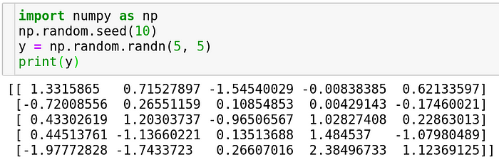
You can specify any number of dimensions to build an array of numbers sampled from a normal distribution. This is used the most when initializing the weights of a neural network. It can also be used in simulations which depend on generation of random numbers like the Monte Carlo Simulation and so on…

Random uniform array

Another distribution which is also commonly used is a random uniform distribution. It is a distribution which weighs every outcome equally. Just like a coin-flip or a case where every outcome has equal probability, this distribution comes in handy. It returns numbers only bound between 0 and 1.

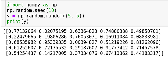
You can specify the number of dimensions as a tuple. Note that it’s not the same as the previous function. In np.random.randn, you are specifying each dimension individually and not as a tuple whereas that’s not the case here.

This could be used to perform coin-flips or events which have definitive probabilities and create a simulation out of the same.

Hope this post helped you become confident with arrays in numpy. In the next post, we will discuss some advanced operations that can be performed on arrays in numpy.

The code snippets above can be viewed on my github in this repository Numpy Explained.

References

• Official Numpy Documentation